Computer Graphics & Geometry

Shader-Based Wireframe Drawing

J. A. Bærentzen,
Informatics and Mathematical Modelling Department of the Technical University of Denmark.

S. L. Nielsen,
Deadline Games, Denmark.

M. Gjøl,
Zero Point Software, Denmark.

B. D. Larsen
Dalux and the Department of Informatics and Mathematical Modelling, Technical University of Denmark.

Contents

1 Introduction
    1.1 Related Work
2 The Single Pass Method
    2.1 Technical Details
        2.1.1 Generic Polygons in Practice
    2.2 Computing the Intensity
3 The ID Buffer Method
4 Implementations and Results
    4.1 Discussion
5 Conclusions and Future Work
References

Abstract

In this paper, we first argue that drawing lines on polygons is harder than it may appear. We then propose two novel and robust techniques for a special case of this problem, namely wireframe drawing. Neither method suffers from the well-known artifacts associated with the standard two pass, offset based techniques for wireframe drawing. Both methods draw prefiltered lines and produce high-quality antialiased results without super-sampling. The first method is a single pass technique well suited for convex N-gons for small N (in particular quadrilaterals or triangles). It is demonstrated that this method is more efficient than the standard techniques and ideally suited for implementation using geometry shaders. The second method is completely general and suited for arbitrary N-gons which need not be convex. Lastly, it is described how our methods can easily be extended to support various line styles.

1 Introduction

We often wish to draw lines on top of opaque polygons. For instance, the problem occurs in non-photorealistic rendering where we may want to draw contours or silhouettes; when we render CAD models, we often want to highlight the edges of patches or polygons or perhaps to show features such as lines of curvature, ridges, or isophotes. One could argue that all of these things are simple to do. However, if we are fastidious and demand lines that are antialiased and of perfectly even width, things become more tricky. It should be pointed out that there is a "right" solution which is to first find the visible set of line segments and then to draw only these segments. Unfortunately, the visible set depends on view direction, and it is costly to recompute for each frame.

Why not simply compute visibility as it is done for polygons by using the depth buffer? This is certainly possible, but it has some limitations. Lines generally do not pass through pixel centers so a line rasterizer merely produces a set of pixel centers which are close to the line - not on it. This is in stark contrast to a polygon rasterizer which produces precisely the set of pixels whose centers are covered by the polygon. Thus, if we resolve visibility by comparing the depth value produced from a line and a depth value produced from a polygon, some issues, which we will discuss later, arise.

However, if we concentrate on a particular case of the problem of drawing lines on polygons, the issues are easier to resolve. In this paper, we focus on wireframe drawing where we wish to draw a polygonal mesh together with the edges of the polygons. Specifically, we propose two new algorithms, which are both designed for modern, commodity graphics hardware supporting fragment and vertex shaders. The algorithms are designed with the goals that they should

support the combination of wireframe and filled polygons.
not suffer from the artifacts of the standard techniques for wireframe drawing.
produce high quality, antialiased lines (without hardware super sampling).

Our first solution is a simple, single pass method which draws the lines as an integral part of polygon rasterization. At little extra effort, the wireframe is drawn using smooth, prefiltered lines [6]. The single pass method is shown in Figure 1b and discussed in Section 2. For hardware supporting geometry shaders, a very efficient implementation is possible.

Figure 1: The top image shows the Stanford Bunny drawn using (a) the offset method with a constant offset, and (b) our single pass method. The bottom image shows the Utah Teapot drawn using (c) a constant offset, (d) our ID buffer method and (e) a slope dependent offset. The white arrows indicate artifacts introduced by the slope dependent offset. Notice the stippling in the constant offset images.

The single pass method is most efficient for convex N-gons for relatively small N. For completely general polygons (not necessarily planar, convex and of arbitrary N) we propose a second method, which we denote the identity (ID) buffer method. This method, which also produces artifact free, prefiltered lines, is shown in Figure 1d and discussed in Section 3. Both our methods can be extended to handle a variety of line styles. Most importantly, we can distance attenuate the line thickness, but many other possibilities present themselves as discussed in Section 4 where our results are presented. Below, we discuss related work, and in the final section (Section 5) we draw conclusions and point to future work.

1.1 Related Work

The standard wireframe rendering techniques are described well in [11]. There is a number of variations, but they all have in common that the filled polygons and the polygon edges are drawn in separate passes. Assuming that the filled polygons have been rendered to the depth buffer, the depth value of a fragment generated from a line (polygon edge) should be either identical to the stored depth value (from a filled polygon) or greater - depending on whether the line is visible or hidden. In reality it is less simple, because the line depth values depend only on the end points whereas the depth value of a fragment that originates from a filled polygon depends on the slope of the polygon. Thus, a fragment produced by polygon rasterization can have a very different depth value from a fragment at the same screen position produced from the line rasterization of one of its edges.

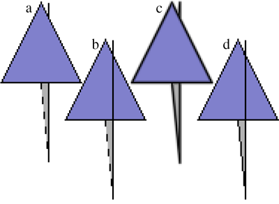
Figure 2: Wireframe drawing using the offset methods (b,d) and our ID buffer method (c) which employs prefiltered lines (and no other method of antialiasing). In (a) no offset has been used, and stippling artifacts are caused by the steep slope of the gray triangle. In (b) a large constant offset (-30000) is used but the result still suffers from stippling artifacts although the edge of the gray triangle penetrates the blue triangle. In (d) a slope dependent offset is used which fixes the stippling but causes disocclusion.

Stippling artifacts where the lines are partly occluded are caused by this issue (Figure 2a). To solve this problem, a depth offset or a shifting of the depth range is used to bias the depth values from either the polygons or the lines to ensure that the lines are slightly in front of the polygons. However, this depth offset has to be very large to avoid stippling in the case of polygons with steep slopes. Hence, in most 3D modeling packages, stippling can still be observed along the edges of polygons with steep slopes. In other cases, the offset is too large and hidden parts of the wireframe become visible. In fact, as shown in Figure 2b, the offset can be both too large and too small for the same polygon. The OpenGL API provides a slope-dependent offset, but this often yields offsets which are too great leading to (usually sporadic) disocclusion of hidden lines as seen in Figure 2d. In the following, we will refer to these methods as offset methods.

A few authors have tried to address the issues in wireframe drawing. Herrell et al. [7] proposed the edging-plane technique. Essentially, this technique ensures that a fragment from a polygon edge is drawn if the corresponding fragment of the filled polygon passed the depth test. This method can be implemented either using special hardware or using the stencil buffer. In any case frequent state changes are required for this method. A variant of the method is discussed in [11]. In Section 3 we propose a similar but more efficient algorithm that requires few state changes. Wang et al. [15] proposed a different technique which explicitly computes occlusion relationships between polygons. While elegant this method cannot be implemented on a GPU and there is no simple way to handle intersecting polygons. Finally, in a method which is most practical for pure quad meshes, Rose et al. [12] encoded signed line distances in textures in order to be able to texture map a detailed mesh onto a simplified model.

In computer graphics, antialiasing is normally performed by taking multiple samples per pixel. These samples are subsequently combined using a simple discrete filter e.g. a straight average [1]. This method is always feasible to implement, but often many samples are required to obtain reasonable quality. Far better quality is obtained if continuous filtering is used. However, this is only possible if we can directly evaluate the convolution of a continuous image with a low pass filter at the point where we desire to compute the intensity of the filtered image. Clearly, this is only possible for filters of finite support, but in the case of lines, Gupta and Sproull [6] observed that the convolution depends only on the distance to the line. Thus, the convolution can be implemented using a 1D lookup table. McNamara et al. [10] proposed an implementation of prefiltered line drawing involving small changes to the fragment generation part of a graphics card, and, more recently, Chan et al. [4] have proposed a method which is implementable on modern graphics cards using fragment shaders. For our second wireframe method (cf. Section 3), we use a similar technique for prefiltered line drawing.

This work is related to Non-Photorealistic Rendering (NPR) in two ways: First of all, both our methods allow for variations of the line style which is also a common feature in NPR systems. Secondly, line drawing (especially silhouette and crease lines) is a central problem in NPR rendering, and wireframe rendering and NPR share the problem of determining the visibility of lines. See [8] for a survey of line drawing in NPR. We use a variation of the ID buffer method from Markosian [9] in order to resolve visibility in our second wireframe method.

The first of the two methods described here was originally presented in a SIGGRAPH sketch [2] based on which NVIDIA implemented a Direct3D 10 version of the method for their SDK [5]. This paper is an expanded version of [3].

2 The Single Pass Method

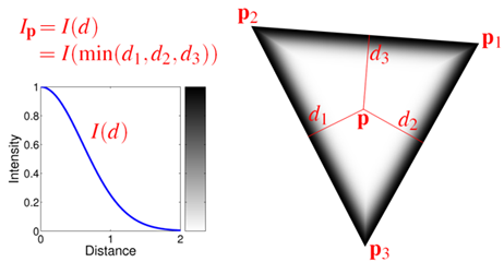
Figure 3: The intensity, I_p, of a fragment centered at p is computed based on the window space distances d₁, d₂, and d₃ to the three edges of the triangle.

In the single pass method, the polygon edges are drawn as an integral part of drawing the filled polygons. For each fragment of a rasterized polygon, we need to compute the line intensity, I(d), which is a function of the window space distance, d, to the boundary of the polygon (see Figure 3) which we assume is convex. The fragment color is computed as the linear combination I(d) C_l + (1−I(d)) C_f where C_l and C_f are the line and face colors, respectively.

Note that a convex N-gon is simply the intersection of N half-planes and that d can be computed as the minimum of the distances to each of the N lines which delimit the half-planes. In 2D the distance to a line is an affine function. Now, suppose, we are given a triangle in 2D window space coordinates, p_i, i ∈ {1,2,3 }. Let d_i = d(p_i) be the distance from p_i to a given line in window space coordinates and let α_i be the barycentric coordinates of a point p with respect to p_i. d is an affine function of p and ∑_i α_i = 1, it follows that

d(p) = d(α₁ p₁ +α₂ p₂ +α₃ p₃) = α₁ d₁ + α₂ d₂ + α₃ d₃ ,

(1)

which has the important implication that we can compute the distance to the line per vertex and interpolate the distance to every fragment using linear interpolation in window space. In the case of triangles, we only need to compute the distance to the opposite edge for every vertex since it shares the two other edges with its neighboring vertices. For quadrilaterals we need the distance to two lines and so on. The distance from a vertex i to the line spanned by the segment jk is computed

d^jk_i =

| (p_j−p_i) ×(p_k−p_i)|

||p_k − p_j||

(2)

2.1 Technical Details

There used to be a slight problem; graphics hardware performs perspective correct interpolation rather than linear interpolation. This problem is fixed by the latest graphics standards (Direct3D and OpenGL) which define a simple linear interpolation mode. However, even when this is not available in the API or supported by the hardware, there is a simple solution: For any datum that requires linear interpolation, we multiply the datum by the vertex w value before rasterization and multiply the interpolated datum by the interpolated 1/w in the fragment stage. This simple procedure negates the effects of perspective correction, and the trick works for arbitrary polygons: Although different modes of interpolation may be used [14], the interpolation is always linear (once perspective correction has been negated) thus affine functions must be reproduced.

In summary, for each vertex of an N-gon, before rasterization we need to

G1 compute the world to window space transformation of all vertices.
G2 compute the distance from vertex i to all edges.
G3 output an N vector d of distances for each vertex. For instance, for a triangle and a given vertex with index i=1, this vector is d′ = [0 d²³₁ 0 ]^T w₁ where d²³₁ is the distance from the first vertex to its opposite line. If non-perspective correct interpolation is not supported, each vector is premultiplied by the w value of vertex i.

After rasterization, i.e. in the fragment shader we receive the interpolated d and

R1 compute the minimum distance: d = min(d¹², d²³, ... , dⁿ¹) (having first multiplied d by the interpolated 1/w if required).
R2 output the fragment color: C = C_l I(d) + (1−I(d)) C_f

Step G1 is generally always performed in the vertex shader. Step G2 should be performed in the geometry shader since the geometry shader has access to all vertices of the polygon (provided it is a triangle). Consequently, if the geometry shader is not used, the vertex shader needs to receive the other vertices as attributes in order to compute the distances. This entails that the application code is not invariant to whether the wireframe method is used, that additional data needs to be transmitted, and, finally, that the use of indexed primitives is precluded since the attributes of a vertex depend on which triangle is drawn. The appendix contains GLSL shader code for hardware which supports geometry shaders and disabling of texture correct interpolation.

One concern was raised in [5]. If one or two vertices of the polygon are behind the eye position in world coordinates, these vertices do not have a well-defined window space position. As a remedy, 2D window space representations of the visible lines are computed and sent to the fragment shader where the distances are computed. While this greatly complicates matters and makes the fragment shader more expensive, the case is rare which entails that the more complex code path is rarely taken.

2.1.1 Generic Polygons in Practice

It would clearly be very attractive to have an implementation of this method which works on arbitrary polygons. This is relatively straightforward, but we must be able to send an arbitrary polygon to the graphics API. If we use OpenGL, the GL_POLYGON primitive is of little use, unless we send all vertices as attributes of every vertex. This is likely to be the least efficient approach.

It is a somewhat better strategy to exploit the fact that a geometry shader can accept "triangles with flaps" as its input. In practice, we use the primitive GL_TRIANGLES_ADJACENCY_EXT and simply use the additional three flap vertices to allow for polygons with up to six sides.

For an almost completely generic approach, we suggest storing the mesh as a texture. One may store the vertices of a polygon in a floating point RGB texture simply by encoding the coordinates as colors. In this case, an N-gon is stored as N consecutive pixels in a texture. We would then render the polygons as points where the vertex defining the point contains the position of the polygon in the texture and the number of edges of the polygon. The work of the geometry shader is then to

look up the vertices of the polygon in the texture.
project the vertices.
compute the distances from each edge to each vertex.

An example of a mesh rendered using this approach is shown in Figure 4. The result is as expected. The method works well as long as polygons are convex and it tends to degrade gracefully for non convex polygons, if we compute absolute distances. To understand this observe that in a convex polygon, the distance to an edge is never negative if we use the convention that the distance is positive on the interior side of an edge. In a concave polygon on the other hand, there must by definition exist a pair points which are interior to the polygon yet on either side of some edge. However, if we use absolute distances, they will both have positive distance to the edge. Thus, linear interpolation of the distance will never produce zero. Consequently, we do not see the extension of an edge passing through the interior of the polygon - unless the extension of the edge happens to touch another vertex (since the vertex would then have distance almost zero to that edge).

Figure 4: Wireframe drawing using the single pass method generalized to arbitrary polygons

Unfortunately, there is another issue with using the single pass method on polygons with many edges. The algorithmic complexity is necessarily on the order of the square of the number of edges since we must compute the distance from each vertex to each edge. This is compounded by the fact that it is much easier to write an efficient geometry shader for the single pass method if it is specialized for triangles. Thus, the generic method used in Figure 4 runs at only 0.4 frames per second even in the case of the Stanford bunny. This is roughly a thousand slower than the specialized version of the algorithm (c.f. Table 1). The enormous difference is due to the increased complexity of the geometry shader and the fact that we cannot use the transform and lighting cache because the mesh is stored in a texture.

Thus, even though it is straightforward to extend the method to polygons with many edges, our recommendation is to use the ID Buffer method presented in Section 3 to handle generic polygons and the single pass method for triangle meshes or quad meshes.

2.2 Computing the Intensity

The convolution of a line and a symmetric filter kernel is a function of distance only in the case of infinite lines. Hence, other methods must be used to handle line segments and junctions of segments. To ensure that lines have rounded end points other authors combine sever al distance functions per line [10], and to compose multiple lines, blending is sometimes used [4]. In this work, we take a slightly different approach and compute the pixel intensity always as a a function, I(d), of the distance, d, to the closest polygon edge.

Thus, our method does not perform prefiltering in the sense of exact continuous domain convolution of a line image and a kernel¹, and, in fact, I is not even a tabulation of convolutions. However, the choice of I is important; I should be a smooth, monotonically decreasing function such that I(0)=1, and I(d_max) ≈ 0 where d_max is the largest value of d that is evaluated. We advocate the use of the GLSL and CG library function exp2. Specifically, we use the intensity function

I=exp₂(−2 d²) ,

(3)

which is never identically 0, but has dropped to 0.011 at d=1.8. We generally find it safe to ignore values for d > 1.8 and set d_max = 1.8. This combination of I and d_max yields lines that appear thin while having very little visible aliasing.

Figure 5: A set of lines of unit width drawn using 4×4 super sampling (left), distance filtering using I(d)=2^−2d2 (middle), and direct convolution with a Gaußian (right).

Figure 5 shows a comparison of three methods, namely 16 times super-sampling (left), our method (in the middle) and prefiltering by direct convolution (right) with a unit variance Gaußian. The Gaußian filter was used by Chan et al. [4]. Another popular filter is the cone function [6,10].

Both our method and Gaußian prefiltering produce lines that are visibly smoother than even 16 times super-sampling. The main difference between our method and direct convolution is that using the latter method the intersections of several lines appear to bulge a bit more. Conversely, our method produces lines that seem to contract slightly where several lines meet (cf. Figure 3). However, both phenomena are perceptible only if I(d) is significantly greater than zero for very large d as in Figure 3.

3 The ID Buffer Method

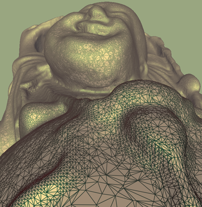
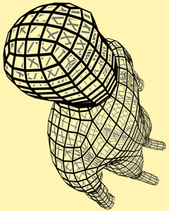
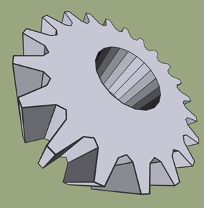
Figure 6: Left: The Happy Buddha model drawn using the single pass method. Center: The single pass method used on a quad mesh. Right: ID buffer method used to draw a gear. Hardware antialiasing (16 times) was used only on the center image (since alpha testing would otherwise introduce aliasing).

The strength of the single pass method is its simplicity and the efficiency which is due to the fact that the method is single pass and requires very little work per fragment. In a generalization to non-convex polygons, more work is required per fragment since the closest polygon feature is sometimes a vertex and not a line. Unfortunately, distance to vertex is not an affine function and it must be computed in a fragment program. Moreover, N-gons for very large N are only possible to handle if they are triangulated. Thus, our generalization of the single pass method works on triangulated N-gons, and unfortunately this means that the quality depends, to some extent, on the triangulation.

Due to these issues, we propose the following method for completely general polygons. The method subsumes a technique for prefiltered line drawing which resembles the one proposed by Chan et al. [4] but differs in important respects:

First of all, Chan et al. use the OpenGL line primitive to generate the fragments covered by the filtered line. In this work, we use a rectangle represented by a quad primitive since there are restrictions on the maximum line thickness supported by OpenGL and even more severe restrictions in the Direct3D API. Second, we compute the intensity based on the distance to the actual line segment whereas Chan et al. and McNamara et al. [10] compute the intensity based on the four distances to the outer edges of the rectangle that represents the line. Our method allows for more precise rounding of the ends of the line segment as shown in Figure 7.

The position of each quad vertex is computed in a vertex program using the following formulas

p₀ = v₀,

p₀.xy + = S (− a − b) t v₀.w

p₁ = v₁,

p₁.xy + = S (+ a − b) t v₁.w

p₂ = v₁,

p₂.xy + = S (+ a + b) t v₁.w

p₃ = v₀,

p₃.xy + = S (− a + b) t v₀.w ,

(4)

where v₀ and v₁ are the line vertices in clip coordinates. t is the line thickness in window coordinates, a and b are unit vectors along and perpendicular to the line in window coordinates and S is a matrix transforming from window to normalized device coordinates from whence scaling by w brings us back to clip coordinates. The terms are illustrated in Figure 7.

The window space positions of v_i are passed to the fragment program where the distance from the fragment center to the line segment is computed. In fact, we only need the square distance for the intensity function (3) which is not costly to compute.

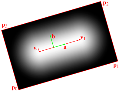
Figure 7: This figure illustrates how a single prefiltered line is drawn. The two endpoints are projected and then the line is made longer and wider in 2D.

When lines are drawn in a separate pass, the problem is to ensure that a line fragment is drawn if the line is the edge of the polygon which is drawn to the same pixel position. For this purpose, an ID buffer - which is simply a window size texture containing unique polygon IDs - is used [9]. Markosian uses a slightly more involved method than we do. In our implementation, we only need to sample the ID buffer in pixel centers which renders the method far simpler than if one needs to sample arbitrary locations in window space. See [9] for details.

The ID buffer is sufficient except in the case where the edge belongs to the silhouette of the object. If a line fragment belongs to a line along the silhouette, the pixel in the ID buffer either contains 0 (background) or the ID of a polygon below the silhouette line. In either case, the line fragment is closer than the polygon below. Hence, we can use the depth buffer without the need for offsetting to distinguish this case.

The method is described succinctly below:

Pass 1: With depth testing and depth buffer updates enabled, each polygon is rendered (filled) with a unique ID as its color attribute. The produced image is the ID buffer.
Pass 2: For each polygon, all edges are drawn using the method discussed above. A given fragment belonging to a line will be written to the framebuffer either if its ID matches the corresponding pixel in the ID buffer or if the depth test is passed. The last condition ensures that silhouette fragments are drawn. The max blending operator is used to ensure that if several fragments pass for a given pixel, the maximum intensity passes. Depth values are not changed during this pass.
Pass 3: At this point, the framebuffer contains alpha values and colors for the lines and depth values for the filled polygons. Now, we draw the filled, shaded polygons with the depth test set to equal. The polygon fragments are combined with the values in the frame buffer using blending. A window filling quad is drawn to perform blending for silhouette pixels.

While the overall approach resembles that of [7], there are important differences: Their method was created for a fixed function pipeline, it did not use prefiltered lines, and the loops have been inverted leading to much fewer state changes and, consequently, greater efficiency. Herrell et al. had to perform all operations for each polygon before moving on.

4 Implementations and Results

	GeForce	Quadro	GeForce	GeForce	GeForce	Geforce
	FX5900XT	FX3000	6600GT	7800 GTX	8800 GTX	8600M GT
Teapot, 6320 triangles
offset	209.31	734.76	363.04	482.68	1548.41	439.76
single	254.22	195.81	589.59	1512.09	6226.87 (5822.38)	327.24 (808.72)
ID	22.51	23.32	87.65	263.37	550.40	86.42
Bunny, 69451 triangles
offset	44.26	138.73	65.12	66.44	176.73	124.39
single	97.68	103.65	146.7	348.22	1506.22 (1344.25)	42.30 (380.16)
ID	4.89	5.13	19.8	61.45	114.58	15
Buddha, 1087716 triangles
offset	3.3	9.96	4.23	4.55	11.28	11.64
single	6.56	7.07	5.31	24.19	102.74 (34.12)	2.98 (42.51)

Table 1: Performance measured in frames per second. The best performing method for each combination of mesh and graphics card is highlighted in red. For the Geforce 8800 GTX and 8600M GT the numbers in parentheses indicate the performance when geometry shaders are used.

The single pass method has been implemented in CG, GLSL and HLSL. The first two implementations are based on the OpenGL API while the last implementation is based on Direct3D 10. The ID buffer method has been implemented in GLSL/OpenGL and HLSL/Direct3D 9.

We have made a number of performance tests based on the OpenGL/GLSL implementations. To make the numbers comparable across platforms, we have restricted ourselves to testing using triangle meshes. For all methods, we strived to use the fastest paths possible. However, in the pre-Geforce 8 series hardware that we tested, the single pass method did not allow for the use of indexed primitives for reasons we have discussed. In all other cases, we used indexed primitives. We also hinted that geometry should be stored directly in the graphics card memory either as a display list or vertex buffer object. All hardware antialiasing was disabled.

Three well known models were used, namely Newell's Teapot (converted to triangles), the Stanford Bunny, and the Stanford Happy Buddha. The models were arranged to approximately fit the viewport (of dimensions 720 × 576) and rotated 360 degrees around a vertical axis in 3142 steps. For each test, an average frame rate was computed based on the wall-clock time spent inside the rendering function.

A variety of hardware was used for testing. We tried to cover a wide range of graphics cards. Restricting the test to a particular machine would have been difficult for compatibility reasons. Instead, the test program was ported to the various platforms: Windows XP, Linux, and Mac OSX. The ID buffer method requires the drawing of a lot of geometry. On some systems that was too much for either a single vertex buffer or display list. Rather than using a special code path for this model, we omitted the test. Note that this problem has nothing to do with the method per se but only with buffer sizes and the amount of geometry.

4.1 Discussion

When judging the results, which are shown in Table 1, one should bear in mind that in order to make a fair performance comparison, no hardware antialiasing was enabled for any of these tests. Arguably, this lends an advantage to the offset method since hardware antialiasing is required to get an acceptable result for this type of method. Despite this, the single pass method outperforms the offset method by a factor of up to seven on the Geforce 8800 GTX. In general, the advantage of the single pass method over the offset method is greater the more recent the graphics card, and this is undoubtedly due to increasing fragment processing power. The offset method is fastest only on the Quadro FX3000 which is perhaps not surprising since this graphics card is intended for CAD users. However, the relative difference is very small for the largest mesh. It is also interesting to note that the ID buffer method, albeit the slowest, performs relatively well on the 7800GTX and 8800 GTX.

The use of geometry shaders for the single pass method makes little difference on the 8800 GTX, but it makes a great difference on the less powerful 8600M GT. The latter system is a MacBook Pro whose drivers supported the disabling of perspective correct interpolation. The 8800 GTX is a WinXP system which did not support this (at the time of testing). However, the 8800 GTX has more stream processors, and stream processing might have been a bottleneck only on the 8600M GT which entails that only this card really would benefit from the reduced load.

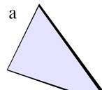
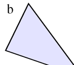
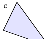
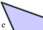
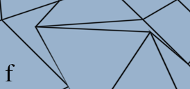
Figure 8: Top: The difference between (a) no disabling of perspective correction, (b) perspective correction disabled using the method described in Section 2, and (c) perspective correction disabled using the Direct3D 10 API. Bottom: The corner of a polygon drawn using (d) the single pass method and (e) the ID buffer method. In (f) non-convex quads are drawn using the single pass method. Notice the fairly graceful degradation.

The single pass method is clearly much faster than the ID buffer method, and while it requires the projected polygons to be convex, it often degrades gracefully in the case of non-convex polygons as shown in Figure 8f. Nevertheless, the ID-buffer is more general since the line rendering is completely decoupled from the polygon rendering. In addition, since the single pass method draws lines as a part of polygon rendering, it is not possible to antialias the exterior side of silhouettes. Figure 8a,b show the corner of a single polygon drawn using both the single pass method and the ID buffer method. The two methods produce results which are, in fact, pixel identical on the inside, but only the ID buffer method draws the exterior part. As this issue affects only silhouette edges, it is rarely noticeable. However, for meshes consisting of few large polygons, the ID buffer method is preferable. Finally, it is possible to first draw the mesh using the single pass method and then overdraw the silhouette edges using the ID buffer method along the lines of [13].

Both proposed methods draw lines of even thickness regardless of the distance or orientation of the polygons. However, an important feature of both our methods is the fact that they are highly configurable. The line intensity is simply a function of distance, and it is possible to modulate the distance or choose a different intensity function. In Figure 9 several different line styles are shown in conjunction with the single pass method.

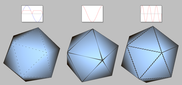
Figure 9: Wireframe drawing using the single pass method and a line thickness which varies as a function of the position along the edge.

Another useful effect (which is not directly possible using the offset method) is to scale the line width as a function of depth. This adds a strong depth cue as seen in Figure 6 center and right. For very dense meshes, it is also useful to fade out the wireframe as a function of distance since the shading of the filled polygons becomes much more visible in this case (see Figure 6 left). Many further possibilities present themselves. For instance, in the center image of Figure 6 alpha is also a function of distance and using alpha testing, most of the interior parts of the quadrilaterals are removed.

5 Conclusions and Future Work

In this paper we have advocated the use of prefiltered lines for wireframe rendering and demonstrated that the prefiltered lines can easily be drawn on the polygons in the pass also employed for rendering the filled polygons. This leads to a simple, single pass method which

is far more efficent than the offset based methods,
does not suffer from the same artifacts,
produces lines which do not need hardware antialiasing, and
can easily be adapted to various line styles.

Our results indicate that the gap between polygon and line rendering is widening and, in terms of performance, the strength of the single pass method is that no line primitive is required.

The ID buffer method is less efficient for triangle and quad meshes, but it handles all cases - including silhouettes - and still at interactive frame rates for meshes such as the Stanford Bunny. For polygons with many edges, the single pass method is also fairly expensive since the distance to each edge must be computed for each vertex of the polygon. Thus, we would recommend using the single pass method for triangles or quads (possibly mixed) but to use the ID buffer method for more complex cases.

References

[1]: Tomas Akenine-Möller and Eric Haines. Real-Time Rendering. A.K. Peters, 2nd edition, 2002.
[2]: J. A. Bærentzen, S. L. Nielsen, M. Gjøl, B. D. Larsen, and N. J. Christensen. Single-pass wireframe rendering, July 2006. Siggraph sketches are single page refereed documents.
[3]: Jakob Andreas Bærentzen, Steen Munk-Lund, Mikkel Gjøl, and Bent Dalgaard Larsen. Two methods for antialiased wireframe drawing with hidden line removal. In Proceedings of the Spring Conference in Computer Graphics, pages 189-195, April 2008.
[4]: Eric Chan and Frédo Durand. Fast prefiltered lines. In Matt Pharr, editor, GPU Gems 2. Addison Wesley, March 2005.
[5]: Samuel Gateau. Solid wireframe. NVIDIA Whitepaper WP-03014-001_v01, February 2007.
[6]: Satish Gupta and Robert F. Sproull. Filtering edges for gray-scale displays. In SIGGRAPH '81: Proceedings of the 8th annual conference on Computer graphics and interactive techniques, pages 1-5, New York, NY, USA, 1981. ACM Press.
[7]: Russ Herrell, Joe Baldwin, and Chris Wilcox. High-quality polygon edging. IEEE Comput. Graph. Appl., 15(4):68-74, 1995.
[8]: T. Isenberg, B. Freudenberg, N. Halper, S. Schlechtweg, and T. Strothotte. A developer's guide to silhouette algorithms for polygonal models. IEEE Computer Graphics and Applications, 23(4):28-37, 2003.
[9]: Lee Markosian. Art-based Modeling and Rendering for Computer Graphics. PhD thesis, Brown University, 2000.
[10]: Robert McNamara, Joel McCormack, and Norman P. Jouppi. Prefiltered antialiased lines using half-plane distance functions. In HWWS '00: Proceedings of the ACM SIGGRAPH/EUROGRAPHICS workshop on Graphics hardware, pages 77-85, New York, NY, USA, 2000. ACM Press.
[11]: Tom McReynolds and David Blythe. Advanced graphics programming techniques using opengl. SIGGRAPH `99 Course, 1999.
[12]: Dirc Rose and Thomas Ertl. Interactive visualization of large finite element models. In T. Ertl, B. Girod, G. Greiner, H. Niemann, H.-P. Seidel, E. Steinbach, and R. Westermann, editors, Proceedings of Vision Modeling and Visualization 2003, pages 585-592. Akademische Verlagegesellschaft, November 2003.
[13]: Pedro V. Sander, Hugues Hoppe, John Snyder, and Steven J. Gortler. Discontinuity edge overdraw. In SI3D '01: Proceedings of the 2001 symposium on Interactive 3D graphics, pages 167-174, New York, NY, USA, 2001. ACM Press.
[14]: Mark Segal and Kurt Akeley. The OpenGL Graphics System: A Specification (Version 2.0). SGI, 2004.
[15]: Wencheng Wang, Yanyun Chen, and Enhua Wu. A new method for polygon edging on shaded surfaces. J. Graph. Tools, 4(1):1-10, 1999.

Appendix: Shaders

In the following, we list the vertex, geometry, and fragment shaders for the variation of the single pass method which employs the geometry shader. Note that almost all complexity is in the geometry shader.


// ------------------ Vertex Shader --------------------------------
#version 120
#extension GL_EXT_gpu_shader4 : enable
void main(void)
{
   gl_Position =  ftransform();
}


// ------------------ Geometry Shader --------------------------------
#version 120
#extension GL_EXT_gpu_shader4 : enable

uniform vec2 WIN_SCALE;
noperspective varying vec3 dist;
void main(void)
{
  vec2 p0 = WIN_SCALE * gl_PositionIn[0].xy/gl_PositionIn[0].w;
  vec2 p1 = WIN_SCALE * gl_PositionIn[1].xy/gl_PositionIn[1].w;
  vec2 p2 = WIN_SCALE * gl_PositionIn[2].xy/gl_PositionIn[2].w;
  
  vec2 v0 = p2-p1;
  vec2 v1 = p2-p0;
  vec2 v2 = p1-p0;
  float area = abs(v1.x*v2.y - v1.y * v2.x);

  dist = vec3(area/length(v0),0,0);
  gl_Position = gl_PositionIn[0];
  EmitVertex();
        
  dist = vec3(0,area/length(v1),0);
  gl_Position = gl_PositionIn[1];
  EmitVertex();

  dist = vec3(0,0,area/length(v2));
  gl_Position = gl_PositionIn[2];
  EmitVertex();

  EndPrimitive();
}


// ------------------ Fragment Shader --------------------------------
#version 120
#extension GL_EXT_gpu_shader4 : enable

noperspective varying vec3 dist;
const vec4 WIRE_COL = vec4(1.0,0.0,0.0,1);
const vec4 FILL_COL = vec4(1,1,1,1);

void main(void)
{
        float d = min(dist[0],min(dist[1],dist[2]));
   float I = exp2(-2*d*d);
   gl_FragColor = I*WIRE_COL + (1.0 - I)*FILL_COL;
}

Footnotes:

¹In fact, that is true of all prefiltering approaches to line drawing due to the mentioned issues related to line segments and the need to handle multiple lines that are intersecting or close together.